Progress bars are pretty much ubiquitous these days; we’ve even seen them on some water coolers. A progress bar provides instant feedback on a given process, so why not bring some of that graphical pizzazz into your spreadsheet, using Excel’s Conditional Formatting feature?
Progress Bars in Excel 2010
“Bar-type” conditional formatting has been around since Excel 2007. But Excel 2007 would only make bars with a gradient – the bar would get paler and paler towards the end, so even at 100% it wouldn’t really look like 100%. Excel 2010 addresses this by adding Solid Fill bars that maintain one color all throughout. These are ideal for creating progress bars.Creating The Bar
The first thing you have to do is enter a numeric value into the cell you’d like to format. You can either enter the value directly or use a formula. In our case I’ll just type it in.
Note how I made the column wider; you don’t necessarily have to do this, but it does help make the bar look more like a “bar” (and not just a colored cell).
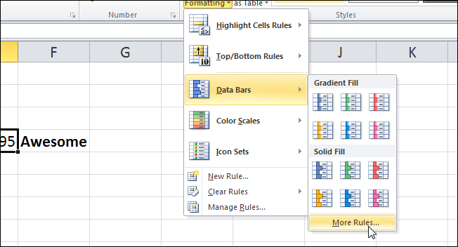
Now click Conditional Formatting, select Data Bars and click More Rules.

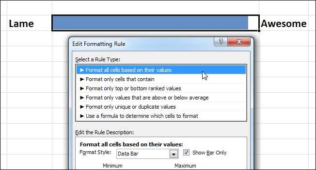
In the New Formatting Rule dialog check the box that says Show Bar Only (so the number doesn’t appear in the cell). Under Minimum and Maximum, select Type as Number. Then, set the Value to the minimum (beginning) value of your scale and maximum (the top of your bar, the end of the process). We’ll just go for 0 and 100, but you could set this to anything that works for you.
Now let’s configure the Bar Appearance. Make sure the Fill is Solid Fill and select the color you’d like to use. When you’re done, the dialog should look similar to this:

Now click OK, and you’re done! At this point you should have a beautiful, crisp progress bar adorning your spreadsheet.
No comments:
Post a Comment